Chapter 3 Three-phase contact lines
Now we consider the mechanics at the intersection of the mutual interfaces between three adjoining immiscible phases, the so-called three-phase contact line. One of the three phases must be a liquid, so that surface tension between this liquid phase and the other two phases are under tension. There are two cases we consider in this chapter: (i) where the three phases are two immiscible liquids and a third fluid, and (ii) where the three phases are liquid, another fluid and a solid. (Here fluid implies either a liquid or a gas.)
3.1 Liquid-liquid-fluid contact line
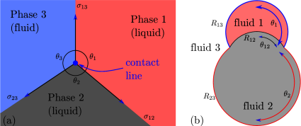
At the three-phase contact line between three fluids (naturally, at least two of these must be immiscible liquids), the action of surface tension must form a Neumann triangle. In other words, the sector angles for the three phases (see Figure 3.1a) must adjust themselves in such a way that the force of surface tension from the three interfaces is balanced. Mathematically, projecting the force along and perpendicular to the 1-3 interface, yields
| (3.1a) | |||
| (3.1b) |
Either equation (3.1) or the geometric interpretation of the Neumann triangle uniquely determine the angles , and , provided the following inequalities are satisfied:
| (3.2a) | ||||
| (3.2b) | ||||
| (3.2c) |
3.1.1 Application: Two drops in contact
The Young-Laplace equation and the Neumann triangle construction is used to determine the geometry of two drops (or bubbles) in contact with each other. The geometry is schematically shown in Figure 3.1(b). The volumes of the two liquid drops ( and ) are known, as are the pairwise surface tensions of the interfaces (, , and ). Each interface takes the shape of a axisymmetric shperical cap. The unknowns of the geometry are the angles (, , ) and the radii (, , ) of the spherical caps, which constitute six unknowns. To determine these six unknowns, we use the following six conditions:
-
1.
The volumes of the two drops depending on the geometry furnish two equations, which are of the form
(3.3a) (3.3b) where is a function that represents the volume of spherical cap of radius and angle .
-
2.
The pressures difference across the three interfaces is given by Laplace pressure, which furnishes one more equations as follows
(3.4a) (3.4b) (3.4c) Here the pressure differences constitute two additional unknowns, which could be eliminated as
(3.5) -
3.
The Neumann triangle condition furnishes two conditions for force balance along two orthogonal directions as
(3.6a) (3.6b) -
4.
Geometric compatibility that radius of the contact line is identical between the three interfaces, which reads
(3.7) These appear to be two more equations, but indeed (3.5), (3.6b) and (3.7) are dependent on each other, with only three independent equations. This is a remarkable observation because it implies that the consideration of Laplace pressure jumps (3.5) arises out of a combination of vertical force balance (3.6b) and geometric compatibility (3.7). This dependence can be understood as combination of a local force balance (leading to Laplace pressure jumps) forming the global force balance on the contact line (i.e. Neumann triangle).
These six independent equations in six unknowns can be solved to determine the resultant geometry of the two-drop complex.
3.2 Solid-liquid-fluid contact line
Considerations change when one of the phases is a rigid solid so its interface with the other phases does not deform. A schematic of this situation is shown in Figure 3.2, where without loss of generality, we denote the third fluid to be air. The surface tension on the liquid-air, solid-liquid and solid-air interfaces is denoted , and , respectively. Since only the liquid-air interface is deformable in this situation, let us say that it makes an angle with the solid surface.
3.2.1 Equilibrium based on energetic considerations
An important variable that determines whether and how the liquid spreads on the solid surface is the differential change in surface excess energy caused by the motion of the interface. If the contact line in Figure 3.2(a) displaces a distance away from the liquid phase, then this contributes to an additional solid-liquid excess energy of , and a reduction in the solid-air excess energy of . However, such a displacement would cause the liquid-air interface to expand a distance , costing an additional excess energy of . Since thermodynamic systems tend to reduce the excess energy, the decrease in excess energy can be considered to be a driving force behind the spreading of the liquid. This quantity may be written in terms of the wetting parameter defined as
| (3.8) |
The decrease in excess energy is .
First, suppose . In this case, the contact line has a tendency to advance (i.e. the liquid wets more surface of the solid) if , and the contact line has the tendency to recede (i.e. the liquid wets less solid surface) if . Equilibrium corresponds to the case between the two tendencies, i.e. . The angle that satisfies this condition is called the equilibrium contact angle, which we will denote . Thus,
| (3.9) |
This relation is called the Young-Dupré relation.
Now, let us consider the case . (The case may be treated by exchanging the roles of liquid and air.) The condition may be interpreted as . If the solid surface is coated by a microscopically thin layer of the liquid, as shown in Figure 3.2(b), the equivalent excess energy of the surface per unit area is . When , this state of the liquid coated solid surface is therefore thermodynamically favourable compared to the pristine solid-air interface. As a consequence, any vapour of the liquid present in the environment spontaneously condenses on the solid surface coating it upto a point where the equivalent excess energy becomes equal to . In this manner, unless extreme care is exercised to maintain the purity of the interface, surfaces with large values of surface excess energy are spontaneously contaminated by chemical elements present in the environment that reduce the equivalent excess surface energy. Thus, for materials which posses , contaminants spontaneously reduce the excess surface energy to an equivalent value of 1. For this reason, the case reduces to the situation (and by argument of exchanging the fluid and the liquid reduces to ).
3.2.2 Equilibrium based on force balance considerations
We now present the same results based on force-balance considerations.
The unbalanced surface tension forces (per unit length perpendicular to the plane of the paper) acting at the contact line is
| (3.10) |
When , i.e. , the unbalanced force points into the liquid and the contact line tends to recede and de-wet the solid, whereas when , i.e. , the unbalanced force points away from the liquid and tends to advance the contact line and the liquid to wet the solid. Equilibrium is attained at when the unbalanced force vanishes.
3.2.3 Contact line motion
Contact lines move in the direction of unbalanced tangential force. The seed with which they move is a topic of current research, but there is no doubt that they move in te direction of unbalanced tangential force, which as argued earlier depends on .
The idealized relations derived in §3.2.2 can only hold for truly flat surfaces. However, real surfaces are rarely flat, which has non-trivial consequences for the motion of the contact line. These consequences are expressed in the literature using terms such as pinning, de-pinning, stick-slip motion, and contact line hysteresis. We present a rationalization of these phenomena here.
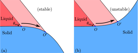
To understand the basic mechanisms, consider the influence of curvature of a solid surface on the tendency of contact line motion. The two possibilities of convex and concave surfaces is shown schematically in Figure 3.3. In the first case, Figure 3.3(a) shows the contact line on a curved solid surface with the convex face towards the liquid. The liquid initially makes an angle equal to the equilibrium contact angle at the contact line. If we now imagine a small displacement of the contact line as shown in this figure, the contact angle changes in such a way as to push the contact line back to its original location. This contact line configuration is stable. However, if the concave face of the solid is towards the liquid, as shown in Figure 3.3(b), the change in contact angle pushes the contact line further away from its initial location. This contact line configuration is unstable and runs away from its original location.
Next we use the background developed so far to discuss the phenomena emerging from the interaction of contact lines with surfaces that possess microscopic features. To illustrate the simplest such phenomena, consider a axisymmetric drop on a surface with a well-defined concentric geometric asperity, such as the one shown in Figure 3.4. The surface is otherwise smooth and offers a fixed equilibrium contact angle to the liquid in the drop. Consider the asperity to be miscroscopic, i.e. of a length scale much smaller than the drop radii in question. Depending on the volume of the deposited liquid, the equilibrium shape of the drop is a spherical cap with a contact-line radius .
Now imagine increasing the volume of the deposited drop on the surface, which advances the contact line. In doing so, the drop volume traverses the path shown in Figure 3.5(a) and the shapes in Figure 3.5(b). For small volumes, the contact line of the deposited drop has a radius smaller than the asperity. As the volume increases and the contact line approaches the asperity, the surface is concave to the liquid and, therefore, unstable. This causes the contact line to slip over a small region, depicted in Figure 3.5(a) from points A to B. On the convex part of the solid surface, the contact line is stable, and offers a range of microscopic orientations to the liquid over the extent of the asperity. This process is depicted in Figure 3.5(a) between points B and C, and the corresponding interface shapes are shown in Figure 3.5(b). As the contact line traverses the asperity, while the microscopic contact angle the liquid surface makes with the local solid surface remains equal to the equilibrium contact angle, the apparent or the “macroscopic” contact angle traverses a range equal to the range of the surface orientation. In this range, the contact line itself moves only by an amount comparable to the asperity scale. For microscopic asperities, the contact line appears to be pinned at the asperity, while the the angle can take a range of values, say , depending on the precise details of the shape of the asperity. If the volume of the drop exceeds beyond that of point C in Figure 3.5(a), the contact line depinns and slips to the position given by D.
Now imagine decreasing the volume below that given by point D, which recedes the contact line. The drop shape then evolves along the geometry described in Figure 3.5(c-d). On the way towards deflating the drop, the path taken by the drop jumps from D’ to C’ and B’ to A’, which is distinct from the path taken while inflating. The contact line pins and depins, but between different positions compared to an advancing contact line. The difference in paths taken by an advancing contact line versus a receding contact line is termed as contact line hysteresis.
A similar picture is expected at chemical asperities on a flat solid surface. A chemical asperity is a region of the surface where the equilibrium contact angle varies from the rest of the surface. Here we state without proof or demonstration that phenomena similar to pinning, depinning, stick-slip behaviour and contact line hysteresis also exists in the presence of chemical asperities.
The roughness of real surfaces is best characterized as random, composed of a distribution of geometric and chemical asperities on the microscale. Because of the roughness, the contact line pins can pin at any location and only advance if the contact angle exceeds a value called the advancing contact angle, which is greater than the equilibrium contact angle on a flat surface. Similarly, the contact line recedes when the contact angle decreases below called the receding contact angle, which is smaller than the equilibrium contact angle.
3.3 Conclusion
In this chapter, we have presented conditions of mechanical equilibrium at the three-phase contact line. The nature of the condition depends on whether all three phases are deformable, or whether one of the three phases is rigid. When one of the phases is rigid, mechanical equilibrium demands the satisfaction of the Young-Dupré relation. However, microscopic geometric and chemical asperities on the rigid surface then lead to phenomona of contact line pinning, depinning, stick-slip and hysteresis. For deformable phases, a Neumann triangle condition on the orientation of the interface applies. In recent years, experiments have confirmed the validity of the Neumann triangle condition for soft solids, such as hydrogels (1).
Another topic we did not discuss in this chapter is that of contact line behaviour on textured surfaces, i.e. surfaces with structured microscopic roughness. Texture systematically changes the energetic considerations of the interface with the solid surface. This leads to the lotus leaf effect, a phenomenon where droplets of water roll off of lotus leafs without wetting the surface. The explanation invokes a state of the interface called the Cassie-Baxter state, where the droplet balances gently on the tips of the microstructure without wetting the whole solid surface. However, the effect could be disrupted by transitioning to the so-called Wenzel state, where the liquid wets the whole surface. We will be seeing much more research on these topic in the coming years.
This completes the preliminaries necessary to mathematically model physical phenomena with liquid interfaces.